BoolForge Tutorial #8: Perturbation and sensitivity analysis of Boolean networks

In this tutorial, we study how Boolean networks respond to perturbations. Rather than implementing perturbations manually, we leverage BoolForge’s built-in robustness and sensitivity measures.

You will learn how to:

• quantify robustness and fragility of Boolean networks under synchronous update,

• interpret basin-level and attractor-level robustness measures,

• compare exact and approximate robustness computations, and

• compute Derrida values as a measure of dynamical sensitivity.

These tools allow us to assess dynamical stability and resilience of Boolean network models in a principled and computationally efficient way.

---

0. Setup

import boolforge
import numpy as np
import pandas as pd
import matplotlib.pyplot as plt

---

1. A running example Boolean network

We reuse the small Boolean network from the previous tutorial.

string = """
x = y
y = x OR z
z = y
"""

bn = boolforge.BooleanNetwork.from_string(string, separator="=")

print("Variables:", bn.variables)
print("Number of nodes:", bn.N)

Variables: ['x' 'y' 'z']
Number of nodes: 3

---

2. Exact attractors and robustness measures

BoolForge provides a single method that computes:

• all attractors,

• basin sizes,

• overall network coherence and fragility,

• basin-level coherence and fragility, and

• attractor-level coherence and fragility.

These quantities are defined via systematic single-bit perturbations in the Boolean hypercube and can be computed exactly for small networks.

results_exact = bn.get_attractors_and_robustness_measures_synchronous_exact()
results_exact.keys()

dict_keys(['Attractors', 'NumberOfAttractors', 'BasinSizes', 'AttractorID', 'Coherence', 'Fragility', 'BasinCoherence', 'BasinFragility', 'AttractorCoherence', 'AttractorFragility'])

print("Number of attractors:", results_exact["NumberOfAttractors"])
print("Attractors (decimal states):", results_exact["Attractors"])
print("Eventual attractor:", results_exact["AttractorID"])

print("Basin sizes:", results_exact["BasinSizes"])
print("Overall coherence:", results_exact["Coherence"])
print("Overall fragility:", results_exact["Fragility"])

Number of attractors: 3
Attractors (decimal states): [[0], [2, 5], [7]]
Eventual attractor: [0 1 1 2 1 1 2 2]
Basin sizes: [0.125 0.5   0.375]
Overall coherence: 0.3333333333333333
Overall fragility: 0.3333333333333333

---

3. Basin-level and attractor-level robustness

Robustness can be resolved at different structural levels. We now inspect basin-specific and attractor-specific measures.

df_basins = pd.DataFrame({
    "BasinSize": results_exact["BasinSizes"],
    "BasinCoherence": results_exact["BasinCoherence"],
    "BasinFragility": results_exact["BasinFragility"],
})

df_attractors = pd.DataFrame({
    "AttractorCoherence": results_exact["AttractorCoherence"],
    "AttractorFragility": results_exact["AttractorFragility"],
})

print("Basin-level robustness:")
display(df_basins)

print("Attractor-level robustness:")
display(df_attractors)

Basin-level robustness:

	BasinSize	BasinCoherence	BasinFragility
0	0.125	0.000000	0.500000
1	0.500	0.333333	0.333333
2	0.375	0.444444	0.277778

Attractor-level robustness:

	AttractorCoherence	AttractorFragility
0	0.000000	0.500000
1	0.333333	0.333333
2	0.666667	0.166667

Interpretation:

• Coherence measures the fraction of single-bit perturbations that do not change the final attractor.

• Fragility measures how much the attractor state changes when a perturbation does lead to a different attractor.

Importantly, attractors are often less stable than their basins, a phenomenon explored in detail in Tutorial #10.

---

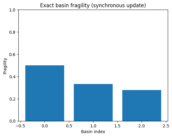
4. Visualization of basin robustness

fig, ax = plt.subplots()

ax.bar(
    np.arange(len(results_exact["BasinSizes"])),
    results_exact["BasinFragility"],
    label="Basin fragility",
)
ax.set_xlabel("Basin index")
ax.set_ylabel("Fragility")
ax.set_title("Exact basin fragility (synchronous update)")
ax.set_ylim(0, 1)

plt.show()

---

5. Approximate robustness for larger networks

For larger networks, exact enumeration of all 2^N states is infeasible. BoolForge therefore provides a Monte Carlo approximation that samples random initial conditions and perturbations.

results_approx = bn.get_attractors_and_robustness_measures_synchronous(
    number_different_IC=500
)

results_approx.keys()

dict_keys(['Attractors', 'LowerBoundOfNumberOfAttractors', 'BasinSizesApproximation', 'CoherenceApproximation', 'FragilityApproximation', 'FinalHammingDistanceApproximation', 'BasinCoherenceApproximation', 'BasinFragilityApproximation', 'AttractorCoherence', 'AttractorFragility'])

print("Lower bound on number of attractors:", results_approx["LowerBoundOfNumberOfAttractors"])
print("Approximate coherence:", results_approx["CoherenceApproximation"])
print("Approximate fragility:", results_approx["FragilityApproximation"])
print("Final Hamming distance approximation:",
      results_approx["FinalHammingDistanceApproximation"])

Lower bound on number of attractors: 3
Approximate coherence: 0.37
Approximate fragility: 0.315
Final Hamming distance approximation: 0.315

Even for this small network, the approximate values closely match the exact ones. For larger networks, these approximations are often the only feasible option.

---

6. Derrida value: dynamical sensitivity

The Derrida value measures how perturbations propagate after one synchronous update. It is defined as the expected Hamming distance between updated states that initially differed in exactly one bit.

derrida_exact = bn.get_derrida_value(EXACT=True)
derrida_approx = bn.get_derrida_value(nsim=2000)

print("Exact Derrida value:", derrida_exact)
print("Approximate Derrida value:", derrida_approx)

Exact Derrida value: 1.0
Approximate Derrida value: 0.9685

Interpretation:

• Small Derrida values indicate ordered, stable dynamics.

• Large Derrida values indicate sensitive or chaotic dynamics.

Derrida values are closely related to average sensitivity of the update functions, and provide a complementary notion of robustness to basin-based measures.

---

7. Summary and outlook

In this tutorial you learned how to:

• compute exact robustness measures for small Boolean networks,

• interpret coherence and fragility at network, basin, and attractor levels,

• approximate robustness measures for larger networks, and

• assess dynamical sensitivity using the Derrida value.

Next steps: In Tutorial #9, we will move from global robustness measures to trajectory-based sensitivity analysis, including damage spreading, Hamming distance dynamics, and time-resolved perturbation experiments.